Injecting gene arrows
Author: Erik Garrison
Synopsis
A pangenome graph represents the alignment of many genome sequences. By embedding gene annotations into the graph as paths, we "align" them with all other paths.
We call this embedding injection.
It's implemented in odgi inject.
Injection makes new paths that are equal to ranges (or alignments) on graph paths.
Of course, these trivially match their source path.
For instance, if we take a gene annotation (e.g. in BED format) on GRCh38, then "inject" it into the graph, we'll get a new path that exactly matches a corresponding sub-path of GRCh38.
However, things get interesting when we use these new gene paths as reference targets for odgi untangle.
Untangling shows us how each query path maps onto a set of targets.
Using our genes as targets will show the order and relative orientation of each path in the graph relative to a set of gene annotations.
This process projects our gene annotations onto overlapping genomes.
In this tutorial, we demonstrate injection and untangling on the human C4 locus.
Our goal is to make gene arrow maps to show the different haplotypes relative to copies of the C4 gene in the GRCh38 reference (C4A and C4B).
We use the gggenes R package to plot gene orders across haplotypes in this locus.
Steps
Build the C4 graph
Assuming that your current working directory is the root of the odgi project, to construct an odgi file from the
C4 dataset in GFA format, execute:
odgi build -g test/chr6.C4.gfa -o chr6.C4.og
The command creates a file called chr6.C4.og, which contains the input graph in odgi format. This graph contains
90 contigs from 88 haploid human genome assemblies from 44 individuals plus the grch38 and chm13 reference sequences.
The contigs cover the Complement Component 4 (C4) region.
In humans, C4 is a protein involved in the intricate complement system, originating from the human leukocyte antigen (HLA) system.
Injecting gene annotations
We start with gene annotations against the GRCh38 reference.
Our annotations are against the full grch38#chr6, in test/chr6.C4.bed:
grch38#chr6  31982057        32002681        C4A
grch38#chr6  31985101        31991058        C4A_HERV-K
grch38#chr6  32014795        32035418        C4B
grch38#chr6  32017839        32023796        C4B_HERV-K
However, the C4 locus graph chr6.c4.gfa is over the reference range grch38#chr6:31972046-32055647.
odgi extract uses PanSN sequencing naming format, and so we can see the
odgi paths -i chr6.C4.gfa -L | grep grc
# grch38#chr6:31972046-32055647
We must adjust the annotations to match the subgraph to ensure that path names and coordinates exactly correspond between the BED and GFA. We do so using odgi procbed, which like Procrustes of Greek mythology cuts BED records to fit within a given subgraph.
odgi procbed -i chr6.C4.gfa -b chr6.C4.bed >chr6.C4.adj.bed
The coordinate space now matches that of the C4A/B subgraph.
# chr6.C4.adj.bed
grch38#chr6:31972046-32055647   10011   30635   C4A
grch38#chr6:31972046-32055647   13055   19012   C4A_HERV-K
grch38#chr6:31972046-32055647   42749   63372   C4B
grch38#chr6:31972046-32055647   45793   51750   C4B_HERV-K
Now, we can inject these into the graph:
odgi inject -i chr6.C4.gfa -b chr6.C4.adj.bed -o - | odgi paths -i - -L | tail -4 >chr6.C4.gene.names.txt
This shows that the annotations have been added as paths (cat chr6.C4.gene.names.txt):
C4A
C4A_HERV-K
C4B
C4B_HERV-K
Their order among the paths is the same as in the input BED.
We can always pipe the output of odgi subcommands to each other, but in this case it will simplify things to save the graph with the injected gene paths:
odgi inject -i chr6.C4.gfa -b chr6.C4.adj.bed -o chr6.C4.genes.og
Visualize the C4 graph with injected gene annotations
To visualize a subset of the graph, execute:
# Select haplotypes
odgi paths -i chr6.C4.genes.og -L | grep 'chr6\|HG00438\|HG0107\|HG01952\|C4' > chr6.C4.selected_paths.txt

odgi viz -i chr6.C4.genes.og -o chr6.C4.genes.selected_paths.png -c 12 -w 100 -y 50 -p chr6.C4.selected_paths.txt -m -B Spectral:4
To obtain the following PNG image:
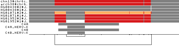
The selected paths (2 reference genomes and 6 haplotypes of 3 individuals) are colored by path depth.
We additionally see the C4 annotation paths at the bottom of the visualization.
Several color palettes are available (see odgi viz documentation for more information), with the default Spectral palette suitable for examining collapsed repeats in the graph.
(Here we use the Spectral:4-color version to increase readability, but Spectral:11 is default with odgi viz -m.)
Human C4 exists as 2 functionally distinct genes, C4A and C4B, which both vary in structure and copy number (Sekar et al., 2016). By injecting annotations into the graph, we can see where these copies fit (bottom 4 path rows in the image above). The longer link on the bottom indicates that the copy number status varies across the haplotypes represented in the pangenome. Moreover, C4A and C4B genes segregate in both long and short genomic forms, distinguished by the presence or absence of a human endogenous retroviral (HERV) sequence, as also highlighted by the short nested link on the left of the image.
Coloring by path depth, we can see that the two references present two different allele copies of the C4 genes,
both of them including the HERV sequence. The entirely grey paths have one copy of these genes. HG01071#2 presents 3 copies of the locus (orange),
of which one contains the HERV sequence (gray in the middle of the orange). In HG01952#1, the HERV sequence is absent.
Untangling to obtain a gene arrow map
We now use the gene names and the gggenes output format from odgi untangle to obtain a gene arrow map!
We use -j 0.5 to filter out low-quality matches.
odgi untangle -R chr6.C4.gene.names.txt -i chr6.C4.genes.og -j 0.5 -t 4 -g \
    | grep '^mol\|HG00438#2\|HG0107\|HG01952#1\|chm13' >chr6.C4.gene.gggenes.tsv
We can then load this into R for plotting with gggenes:
require(ggplot2)
require(gggenes)
x <- read.delim('chr6.C4.gene.gggenes.tsv')
ggplot(x, aes(xmin=start, xmax=end, y=molecule, fill=gene, forward=strand)) + geom_gene_arrow()
ggsave('c4.gggenes.subset.png', height=1.5, width=15)
To obtain the following PNG image:
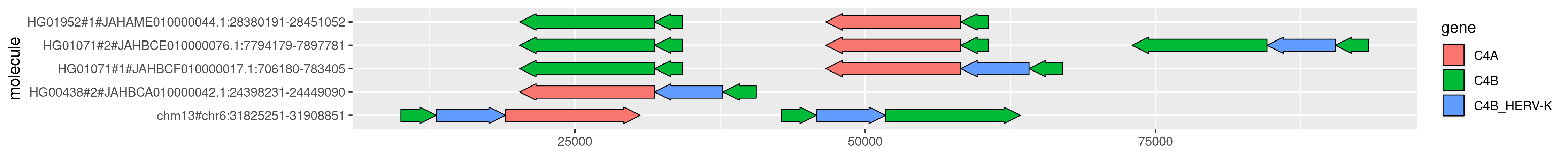
It looks a bit... odd! This is because some of the paths are in the reverse complement orientation relative to the annotations.
We can clean this up by using odgi flip, which flips paths around if they tend to be in the reverse complement orientation relative to the graph.
odgi flip -i chr6.C4.genes.og -o - -t 4 \
    | odgi untangle -R chr6.C4.gene.names.txt -i - -j 0.5 -t 4 -g \
    | grep '^mol\|HG00438#2\|HG0107\|HG01952#1\|chm13' >chr6.C4.gene.gggenes.tsv
We can plot this using the exact same R snippet above:
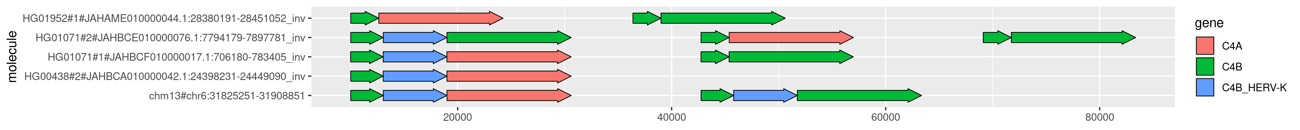
This is somewhat easier to understand.
We're seeing things relative to the forward strand of the graph now, which happens to be sorted according to the GRCh38 reference that is the basis of the C4 annotations we're using.
(n.b. We can ensure this kind of ordering using odgi groom and a reference path.)
We can also do more than just a subset:
odgi flip -i chr6.C4.genes.og -o - -t 4 \
    | odgi untangle -R chr6.C4.gene.names.txt -i - -j 0.5 -t 4 -g >chr6.C4.gene.gggenes.tsv
And plotting with a slightly different ggsave command:
x <- read.delim('chr6.C4.gene.gggenes.tsv')
ggplot(x, aes(xmin=start, xmax=end, y=molecule, fill=gene, forward=strand)) + geom_gene_arrow()
ggsave('c4.gggenes.all.png', height=15, width=15)
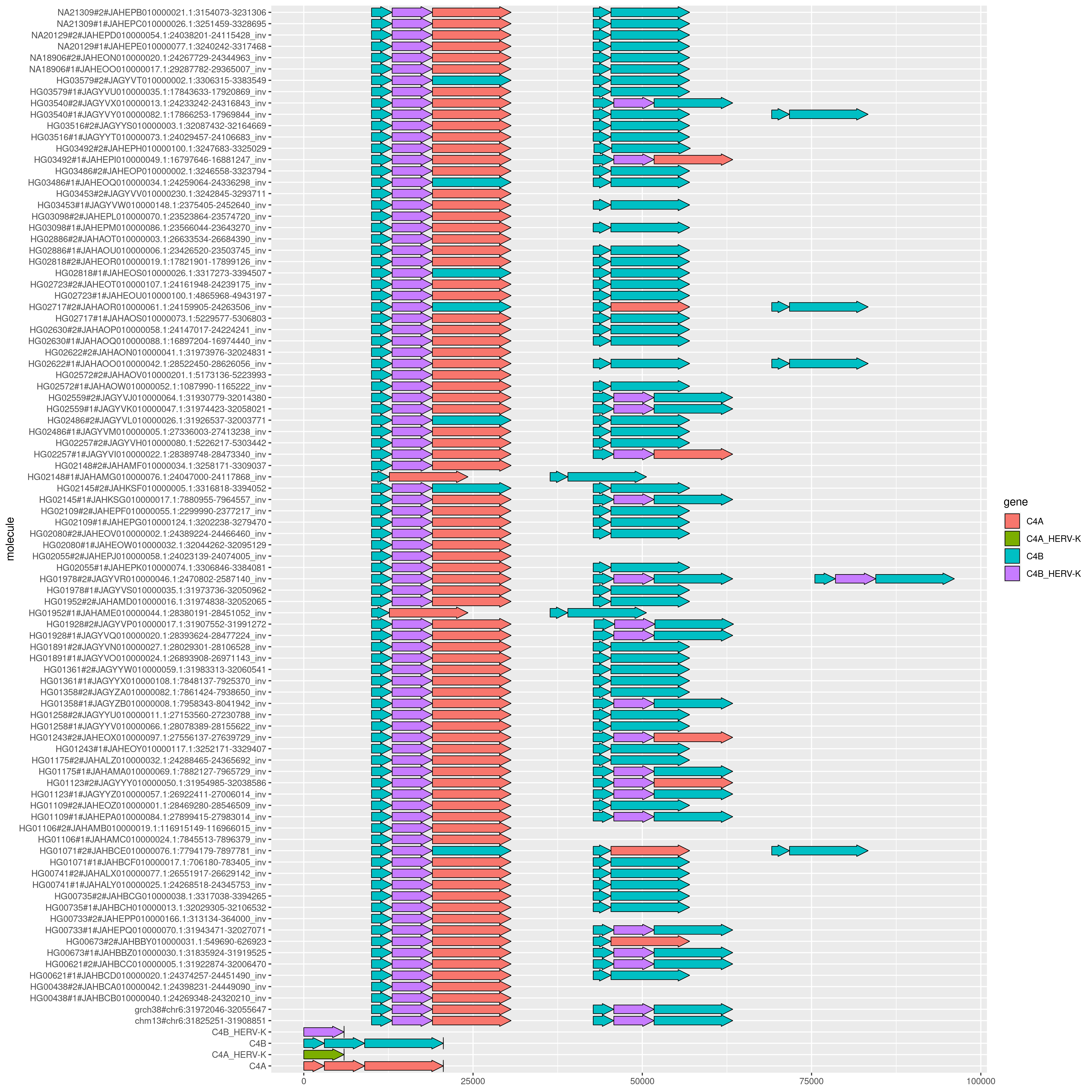
It's surprising that we don't get any matches to the C4A HERV.
Actually, what's happening is simply that the HERVs in GRCh38 are exactly the same.
We can see this by extracting the FASTA corresponding to each, and comparing with sha256sum:
# extract FASTA of paths
odgi paths -i chr6.C4.genes.og -f >chr6.C4.genes.og.fa
# index
samtools faidx chr6.C4.genes.og.fa
# extract HERV-specific sequences and take their sha256sum
samtools faidx chr6.C4.genes.og.fa C4A_HERV-K C4B_HERV-K -n 100000000 \
    | grep -v "^#" | while read f; do echo $f | sha256sum; done
We get the same hash, indicating that this is an exact repeat in the GRCh38 reference.
253f6ea1f8f063c340fce457e88dcd9db8f73bf574544b177976128ba758a811  -
253f6ea1f8f063c340fce457e88dcd9db8f73bf574544b177976128ba758a811  -
While surprising, this explains our arrow map results.