Untangling the pangenome
Author: Andrea Guarracino
Synopsis
A pangenome graphs is a representation of the alignment (or homology) relationships between the sequences represented.
Navigating and understanding the graph requires coordinate systems that we can use to link other data into the graph model,
and thus to all genomes in the pangenome. odgi's tools use the embedded sequences to provide a universal coordinate space
that is graph-independent, thereby remaining stable across different graphs built with the same genomes.
Steps
Build the C4 graph
Assuming that your current working directory is the root of the odgi project, to construct an odgi file from the
C4 dataset in GFA format, execute:
odgi build -g test/chr6.C4.gfa -o chr6.C4.og
The command creates a file called chr6.C4.og, which contains the input graph in odgi format. This graph contains
90 contigs from 88 haploid human genome assemblies from 44 individuals plus the grch38 and chm13 reference sequences.
The contigs cover the Complement Component 4 (C4) region.
In humans, C4 is a protein involved in the intricate complement system, originating from the human leukocyte antigen (HLA) system.
Visualize the C4 graph
To visualize a subset of the graph, execute:
# Select haplotypes
odgi paths -i chr6.C4.og -L | grep 'chr6\|HG00438\|HG0107\|HG01952' > chr6.C4.selected_paths.txt

odgi viz -i chr6.C4.og -o chr6.C4.selected_paths.png -c 12 -w 100 -y 50 -p chr6.C4.selected_paths.txt -m -B Spectral:4
To obtain the following PNG image:
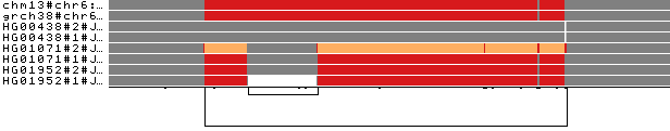
The selected paths (2 reference genomes and 6 haplotypes of 3 individuals) are colored by path depth.
Several color palettes are available (see odgi viz documentation for more information).
Using the Spectra color palette with 4 levels of path depths, white indicates no depth, while grey, red, and yellow indicate depth 1, 2, and greater than or equal to 3, respectively.
Human C4 exists as 2 functionally distinct genes, C4A and C4B, which both vary in structure and copy number (Sekar et al., 2016). The
longer link on the bottom indicates that the copy number status varies across the haplotypes represented in the pangenome.
Moreover, C4A and C4B genes segregate in both long and short genomic forms, distinguished by the presence or absence of a
human endogenous retroviral (HERV) sequence, as also highlighted by the short nested link on the left of the image.
Coloring by path depth, we can see that the two references present two different allele copies of the C4 genes,
both of them including the HERV sequence. The entirely grey paths have one copy of these genes. HG01071#2 presents 3 copies of the locus (orange),
of which one contains the HERV sequence (gray in the middle of the orange). In HG01952#1, the HERV sequence is absent.
Linearize the C4 region
To obtain a more precise overview of a collapsed locus, we can apply odgi untangle to segment paths into linear segments
by breaking these segments where the paths loop back on themselves. In this way, we can obtain information on the copy
number status of the sequences in the locus.
To untangle the C4 graph, execute:
(echo query.name query.start query.end ref.name ref.start ref.end score inv self.cov n.th |
  tr ' ' '\t'; odgi untangle -i chr6.C4.og -r $(odgi paths -i chr6.C4.og -L | grep grch38) --threads 2 -m 256 -P |
  bedtools sort -i - ) | awk '$8 == "-" { x=$6; $6=$5; $5=x; } { print }' |
  tr ' ' '\t'   > chr6.C4.untangle.bed
Take a look at the rows in the chr6.C4.untangle.bed file for the HG00438 and `HG01071 individuals:
cat <(head chr6.C4.untangle.bed -n 1) <(grep 'HG00438\|HG01071' chr6.C4.untangle.bed) | column -t
query.name                                     query.start  query.end  ref.name                       ref.start  ref.end  score     inv  self.cov  n.th
HG00438#1#JAHBCB010000040.1:24269348-24320210  0            9520       grch38#chr6:31972046-32055647  83302      74068    0.966446  -    1         1
HG00438#1#JAHBCB010000040.1:24269348-24320210  9520         42026      grch38#chr6:31972046-32055647  74068      41573    0.997327  -    1         1
HG00438#1#JAHBCB010000040.1:24269348-24320210  42026        50046      grch38#chr6:31972046-32055647  8685       0        0.890347  -    1         1
HG00438#2#JAHBCA010000042.1:24398231-24449090  0            9520       grch38#chr6:31972046-32055647  83302      74068    0.96521   -    1         1
HG00438#2#JAHBCA010000042.1:24398231-24449090  9520         42023      grch38#chr6:31972046-32055647  74068      41573    0.996989  -    1         1
HG00438#2#JAHBCA010000042.1:24398231-24449090  42023        50043      grch38#chr6:31972046-32055647  8685       0        0.890561  -    1         1
HG01071#1#JAHBCF010000017.1:706180-783405      0            9520       grch38#chr6:31972046-32055647  83302      74068    0.966446  -    1         1
HG01071#1#JAHBCF010000017.1:706180-783405      9520         35658      grch38#chr6:31972046-32055647  74068      41573    0.800215  -    1.98971   1
HG01071#1#JAHBCF010000017.1:706180-783405      35658        36005      grch38#chr6:31972046-32055647  41573      41214    0.955679  -    1.43228   1
HG01071#1#JAHBCF010000017.1:706180-783405      36005        68397      grch38#chr6:31972046-32055647  41214      8685     0.991564  -    1.79862   1
HG01071#1#JAHBCF010000017.1:706180-783405      68397        76409      grch38#chr6:31972046-32055647  8685       0        0.88752   -    1.01872   1
HG01071#2#JAHBCE010000076.1:7794179-7897781    0            9520       grch38#chr6:31972046-32055647  83302      74068    0.96624   -    1         1
HG01071#2#JAHBCE010000076.1:7794179-7897781    9520         35659      grch38#chr6:31972046-32055647  74068      41573    0.80019   -    2.98217   1
HG01071#2#JAHBCE010000076.1:7794179-7897781    35659        36006      grch38#chr6:31972046-32055647  41573      41214    0.955679  -    2.43516   1
HG01071#2#JAHBCE010000076.1:7794179-7897781    36006        62028      grch38#chr6:31972046-32055647  74068      41573    0.796543  -    2.99239   1
HG01071#2#JAHBCE010000076.1:7794179-7897781    62028        62375      grch38#chr6:31972046-32055647  41573      41214    0.955679  -    2.43516   1
HG01071#2#JAHBCE010000076.1:7794179-7897781    62375        94764      grch38#chr6:31972046-32055647  41214      8685     0.992205  -    2.59814   1
HG01071#2#JAHBCE010000076.1:7794179-7897781    94764        102786     grch38#chr6:31972046-32055647  8685       0        0.889077  -    1.03765   1
For each segment in the query (query.name, query.start, and query.end columns), the best match on the reference is reported
(ref.name, ref.start, and ref.end), with information about the quality of the match (score), the strand (inv),
the copy number status (self.cov), and its rank over all possible matches (n.th).
To obtain a visualization of the output for the HG00438 and `HG01071 individuals, execute:
library(ggplot2)
x <- read.table('chr6.C4.untangle.bed', sep = '\t', header = T, comment.char="$")
x$query.name <- gsub(":.*","",x$query.name)
x$query.name <- gsub("#J.*","",x$query.name)

ggplot(
  subset(x, query.name %in% c(
    "grch38#chr6",
    "HG00438#1",
    "HG00438#2",
    "HG01071#1",
    "HG01071#2"
    )
  ), aes(x=query.start, xend=query.end, y=ref.start, yend=ref.end)) +
    geom_segment(size=0.3) +
    facet_grid(. ~ query.name) +
    coord_fixed() +
    theme(
      text = element_text(size = 12.6),
      axis.text.x = element_text(size = 12, angle = 90),
      axis.text.y = element_text(size = 12),
    )  +
      xlab("Query start") +
      ylab("Reference start")

ggsave('chr6.C4.untangle.png', width = 32, height = 8,  units = "cm", dpi = 300,  bg = "transparent")
To obtain the following PNG image:
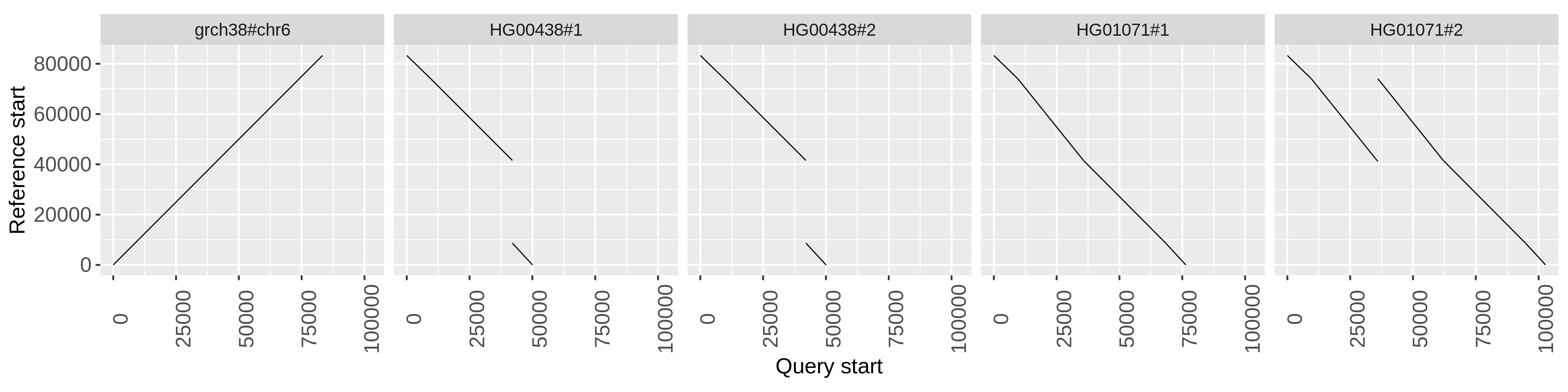
The plots show the copy number status of the haplotypes in the C4 region with respect to the grch38 reference sequence.
On the grch38 reference, C4A precedes C4B, and both are in single copy.
odgi untangle's output makes then clear, for example, that in HG00438 the C4A gene is missing in both haplotypes, while HG01071#2
has two copies of C4B.